Step-by-step guide
Dissolved oxygen (DO) is one of the most common metrics in water quality:
- Serves as a valuable indicator of river health, since all aquatic life depends on oxygen.
- The levels of dissolved oxygen in water are influenced by its physical, chemical, and biochemical activities.
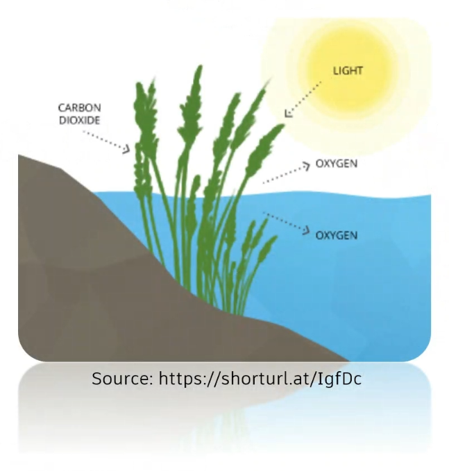
- Oxygen only has solubility in water when it is in equilibrium with air. The saturation value, influenced by temperature (T) and salinity (S), represents the maximum amount of oxygen that can dissolve in water.
- Oxygen levels in water stabilize based on the surrounding oxygen solubility.
In the absence of a pollutograph profile, saturated DO will be derived from the constant temperature and salinity (salt parameters > Constant Concentration (kg/m³)) values defined in the water quality parameters.
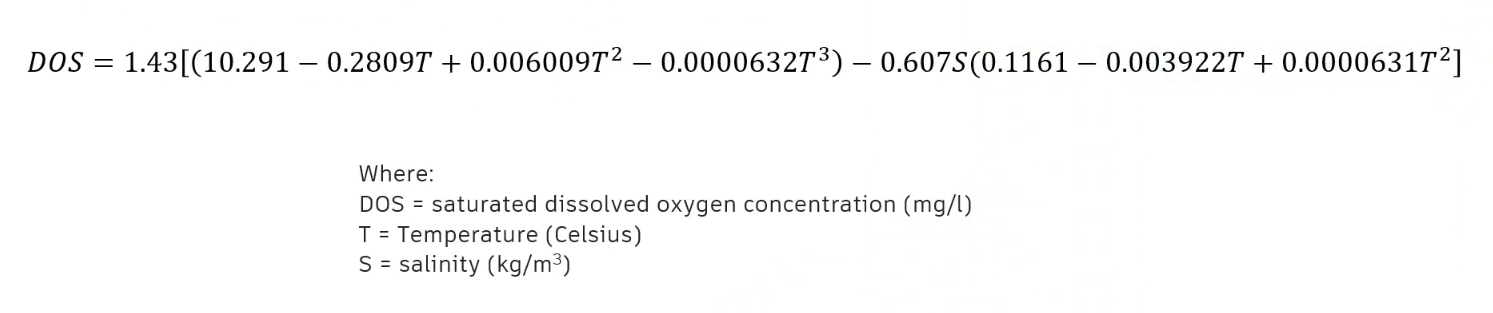
This equation allows for the modeling of dissolved oxygen in a water system:
- Yields the saturated dissolved oxygen concentration value, or DOS.
- Applied in ICM by defining the constant salinity and constant temperature values within the Water quality and sediment parameters.
Dissolved oxygen example scenarios:
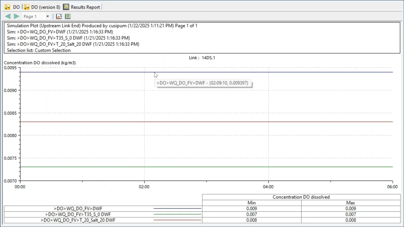
- The first scenario, with a temperature of 20 degrees Celsius and a salinity of 0, yielded a dissolved oxygen saturated value of 0.0093 kilograms per cubic meter.
- In the second scenario, a temperature of 20 and a salinity of 20 resulted in a DOS of 0.0083 kilograms per cubic meter.
- And in the third scenario, a temperature of 35 degrees and a salinity of 0 resulted in a DOS of 0.0073 kilograms per cubic meter.
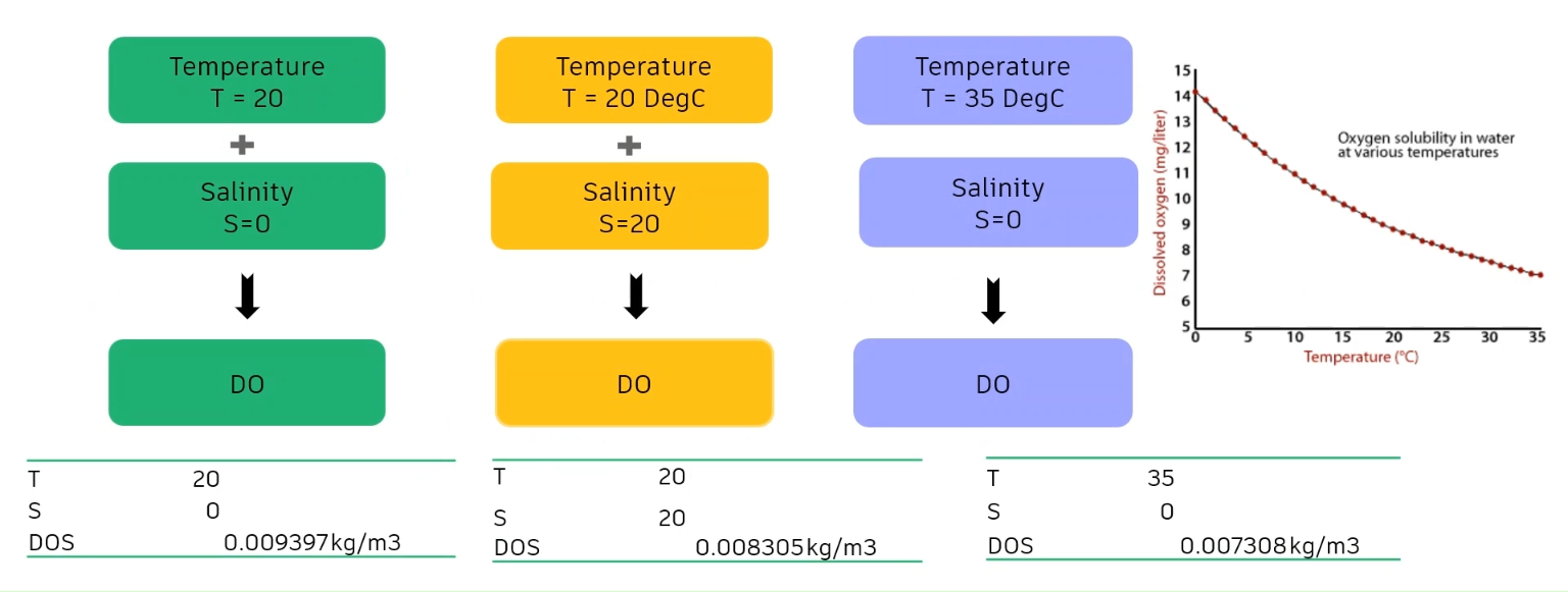
These results demonstrate that dissolved oxygen decreases when the temperature increases. It also shows that the DOS decreases as the salinity increases.
In ICM, to model dissolved oxygen as a function of temperature and salinity in a one-dimensional river:
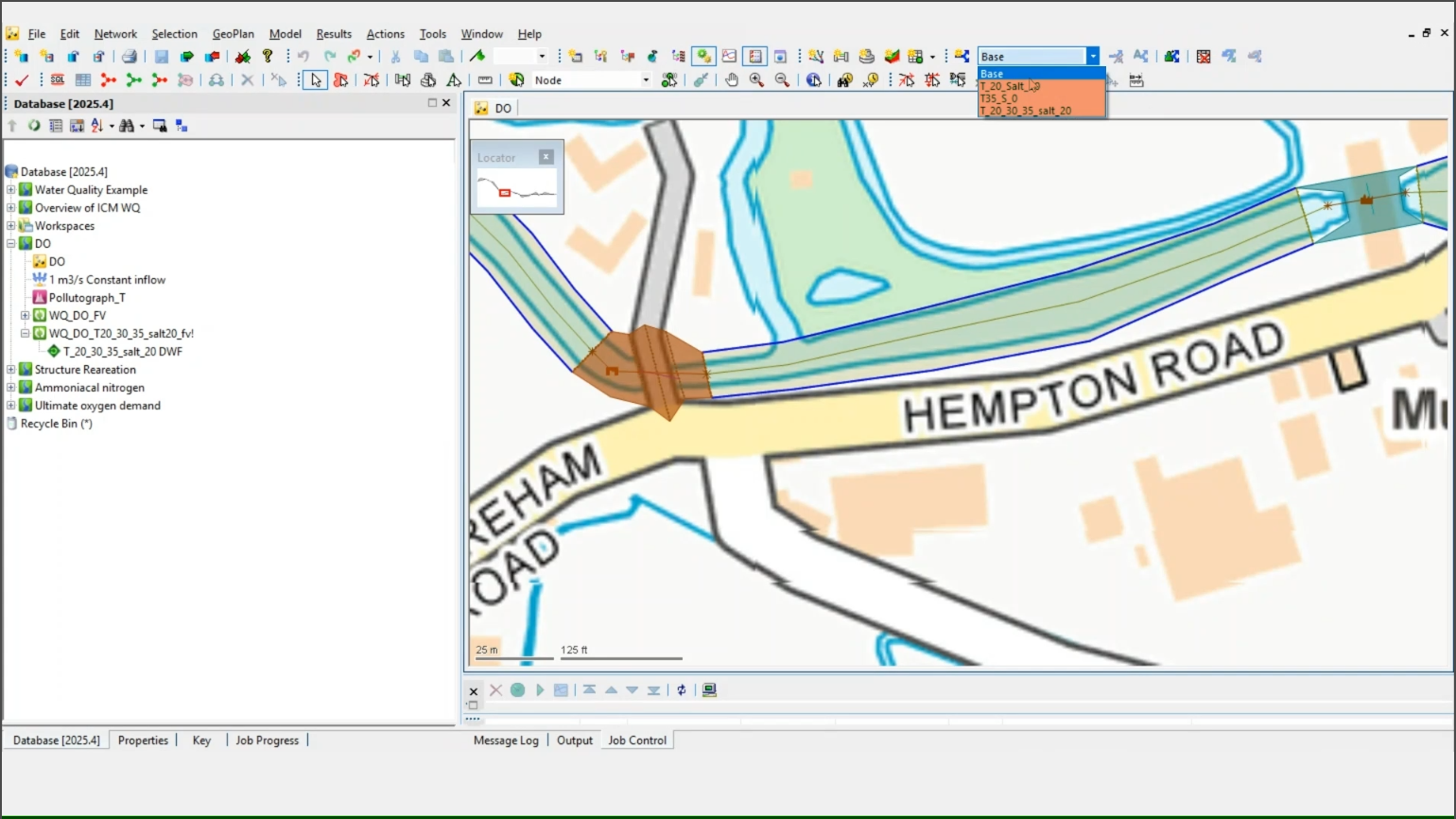
- In the toolbar, expand Scenarios. (Three scenarios are already created for this example.)
- Select the Base scenario.
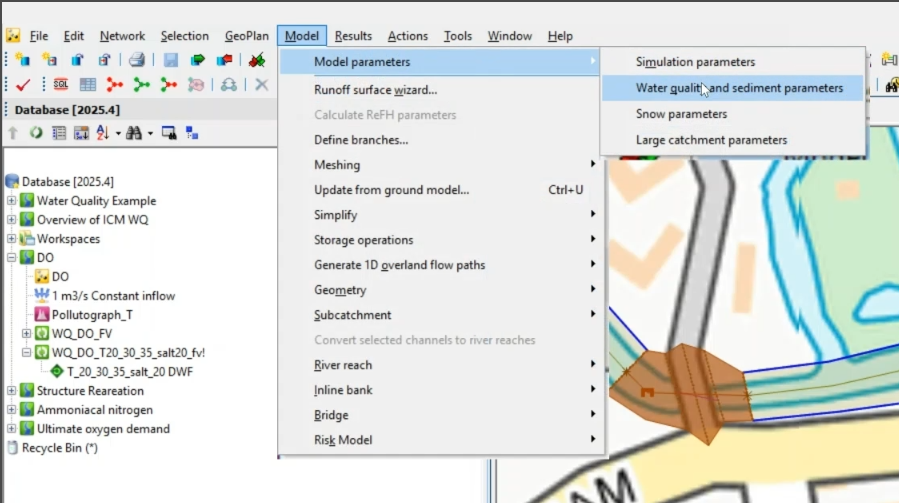
- To review the salinity and temperature parameters, navigate to Model > Model parameters > Water quality and sediment parameters.
- In the Object Properties, under Temperature parameters, set the Constant temperature to 20.
- Under Salt parameters, set the Constant concentration to 0.
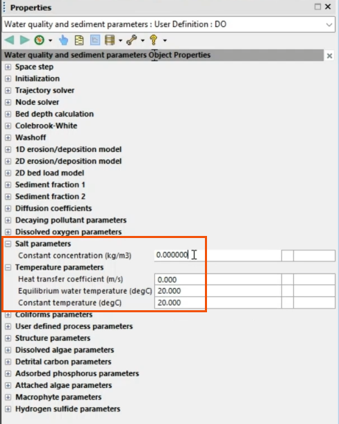
This creates the first scenario.
- Follow the same steps to create the remaining two scenarios, naming them appropriately.
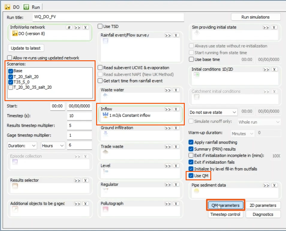
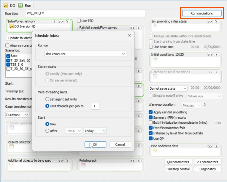
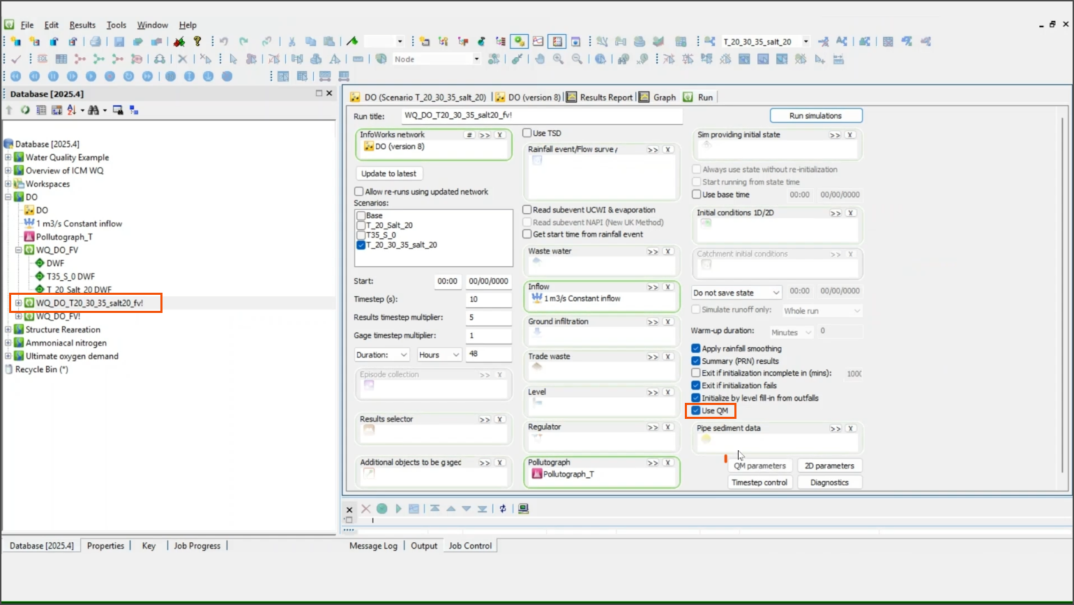
- With the three scenarios created, open the Run dialog.
Note that an inflow hydrograph is being used.
- Specify the water quality option by ensuring that the Use QM option is enabled.
- Click QM parameters.
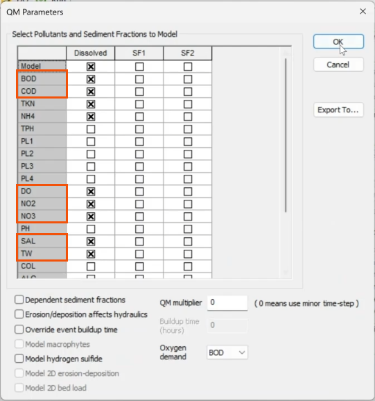
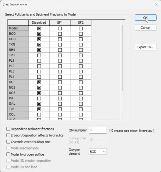
A list of pollutants displays in the QM Parameters dialog.
- Select the appropriate pollutants, such as DO, BOD, COD, NO2, NO3, SAL, and TW.
- Click OK.
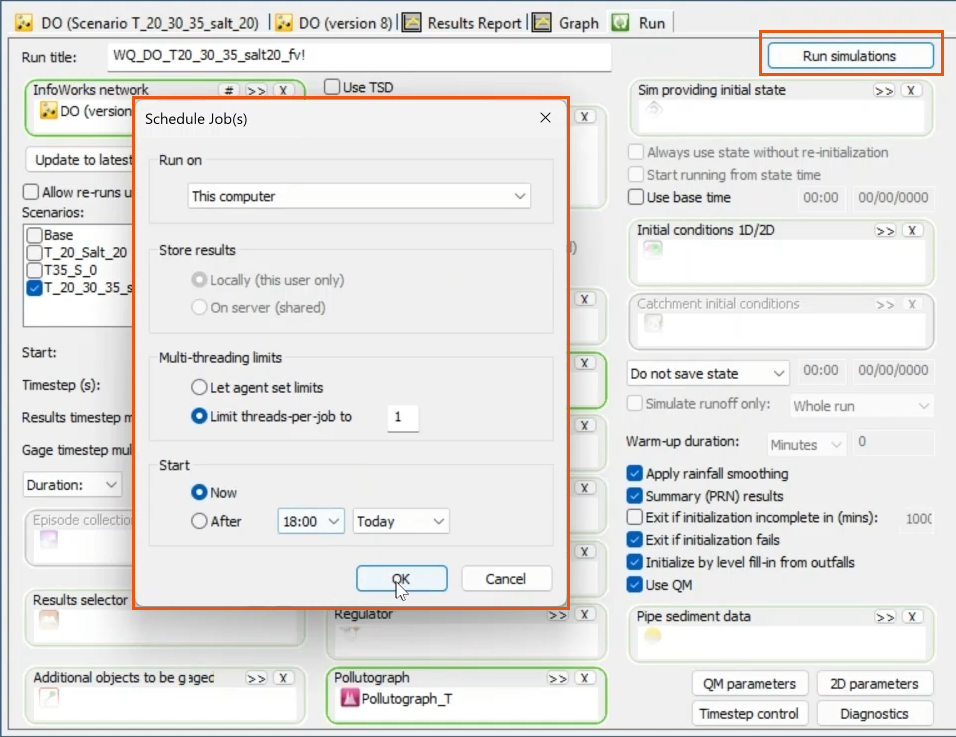
- Back in the Run dialog, click Run simulations.
- In the Schedule Jobs dialog, confirm that all information is correct for the simulations, and then click OK.
Once the simulations are complete, analyze the results; focus on dissolved oxygen profiles along the river reach to observe the effects of water solubility on DO concentration.
To plot all three scenarios on a single graph:
- Select the river reach.
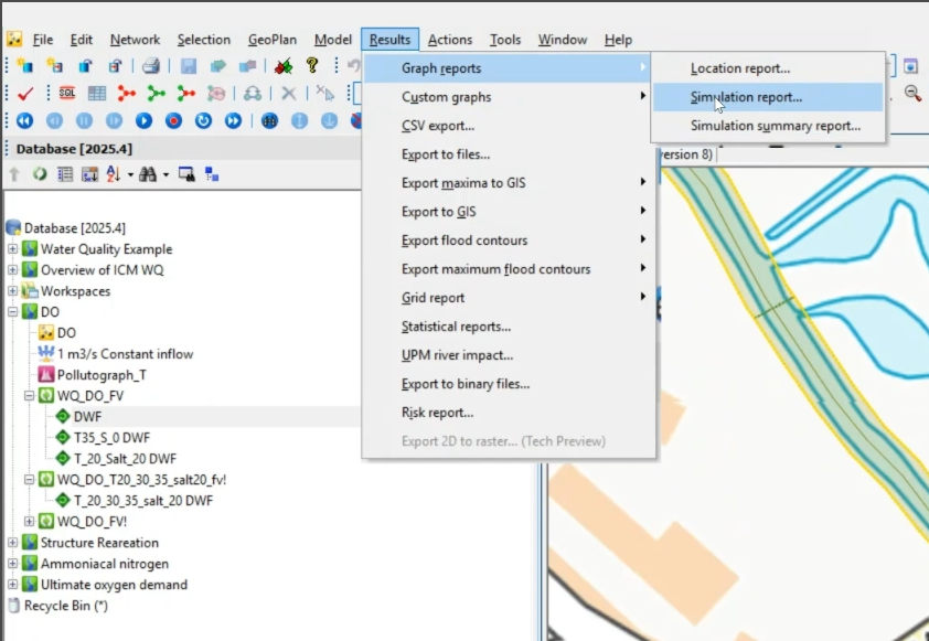
- Navigate to Results > Graph reports > Simulation report.
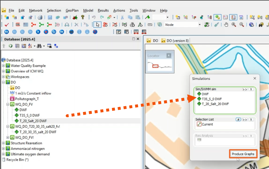
- Drag the three scenarios from the Explorer into the Simulations dialog.
- Specify the object to be graphed, such as the river reach. Here, Current is selected to include the currently selected object.
- Click Produce Graphs.
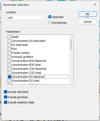
- In the Parameter Selection dialog, select Concentration DO dissolved.
- Click OK.
- Close the Simulations dialog, if it is still open.
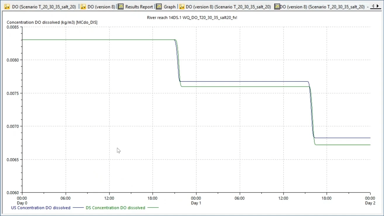
In the graph, the results show that dissolved oxygen decreases as temperature increases. For instance, at 20 degrees Celsius and 0 salinity, DO remains constant at 0.0093 kilograms per cubic meter; and at 35 degrees and 0 salinity, DO is 0.0073 kilograms per cubic meter.
To reproduce the dissolved oxygen profile using a pollutograph:
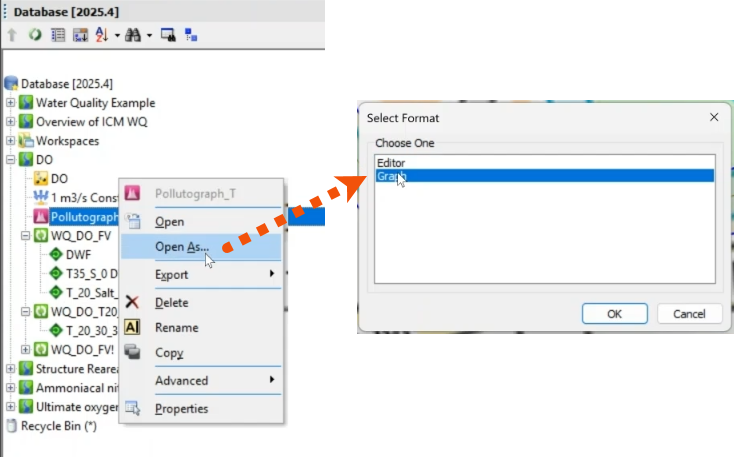
- In the Explorer, right-click Pollutograph_T, which was created previously, and select Open As.
- In the Select Format dialog, select Graph.
- Click OK.
Set the temperature to vary over time while keeping salinity constant at 20 kilograms per cubic meter. This is done by editing the TW tab within the pollutograph.
- Open the Run dialog.
- Select Use QM.
- Click QM parameters.
- In the QM Parameters dialog, select the same list of pollutants used previously.
- Click OK.
- Back in the Run dialog, click Run simulations.
- Confirm the information in the Schedule Jobs dialog, and then click OK.
- On the Results toolbar, click Graph.
- In the Graph dialog, select Concentration DO dissolved (kg/m³).
- Click OK.

The result illustrates how dissolved oxygen decreases as the temperature increases from 20 to 35 degrees Celsius.