Understand and calculate reaeration rates

Step-by-step guide

Reaeration is the process by which oxygen in the air dissolves into water bodies.

• This natural mechanism is essential for maintaining ecological balance and supporting aquatic life.
• Effectiveness of reaeration is constrained by the saturation concentration of oxygen in the water.

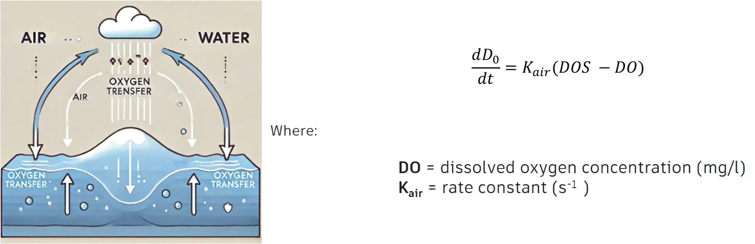
The rate at which reaeration occurs is primarily determined by the oxygen deficit, which is the difference between current dissolved oxygen levels and the saturation concentration.

• Influenced by temperature and hydraulic factors, such as water depth, flow velocity, and salinity.
• Each of these factors significantly impacts the dissolution of, and the distribution of, oxygen within a water body.

The reaeration rate coefficient represents the speed at which oxygen is absorbed into the water, with a typical range of 0.03–0.1 meters per hour.

The reaeration temperature coefficient represents how the transfer velocity changes with temperature, typically benchmarked at 20 degrees C.

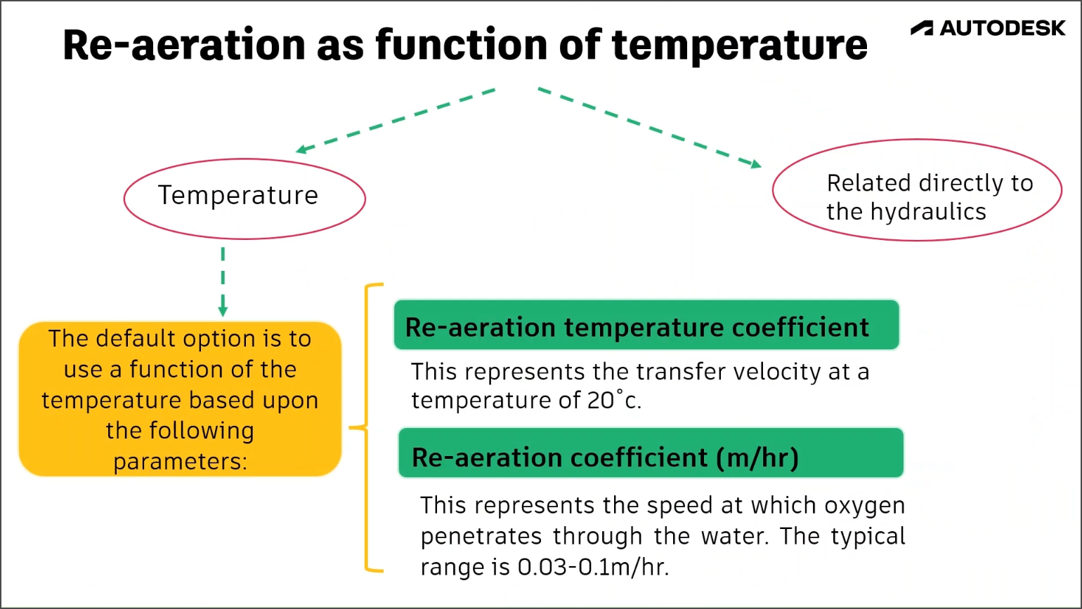
Reaeration as a function of hydraulic variables

Empirical equations are also used to calculate reaeration rates, such as Covar’s 1976 equation.

This method estimates the reaeration rate (K_air) based on hydrodynamic parameters, such as water velocity (u), water depth (h), and temperature (T), using the following equation:

K_air = u 𝛥h/T

To calculate the reaeration rate, select one of these three equations in ICM, based on the water depth, velocity, and temperature:

• For water depths less than 0.61 meters, use the Owens-Gibbs formula:
  K_air = 5.32u^0.67/(d^1.85)
  where:
  K_air = reaeration rate (d^-1)
  u = absolute velocity (m/s)
  d = hydraulic mean depth (m)
• For water depths greater than a specific function of velocity (3.45u^2.5), use the O'Connor-Dobbins formula:
  K_air = 3.930u^0.5/(d^1.50)
• If neither of these two conditions apply, use the Churchill equation:
  K_air = 5.026u/(d^1.67)

For this example, create two scenarios: one to model reaeration as a function of a predefined reaeration coefficient, and one that is based on hydraulic variables. The simulation results can then be compared to show the impact of aeration.

IMPORTANT: This process is limited by the saturation concentration and is proportional to the oxygen deficit, which is the difference between the saturation concentration and the actual concentration level.

First, create a scenario to model reaeration as a function of a predefined reaeration coefficient.

1. Begin with a new scenario called "Reaeration". In this case, it is already created.
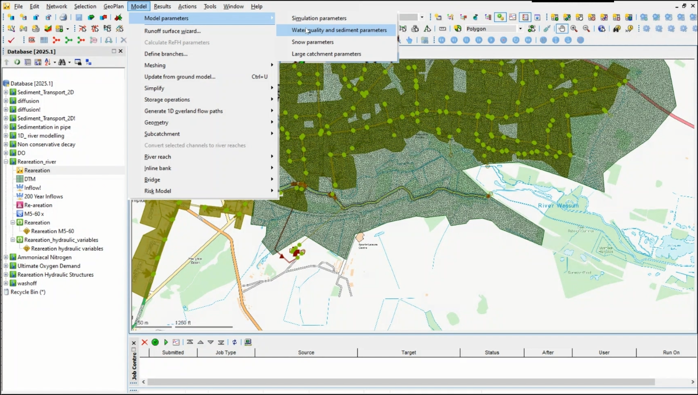
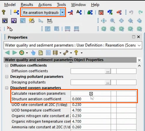
2. Navigate to Model > Model parameters > Water quality and sediment parameters.

3. In the Properties panel, scroll down to Dissolved oxygen parameters and make sure that Calculate reaeration parameters is deselected.
4. Set the Reaeration coefficient to 0.03 meters per hour.

This represents the speed at which a front of oxygen penetrates through the water depth. The stronger the mixing processes, the higher this value will be.

5. Create a pollutograph; or, in this case, open the already created pollutograph named Re-aeration.
6. Select the DO tab.
7. Generate a new event.
8. Assign it a dissolved oxygen value of 0.
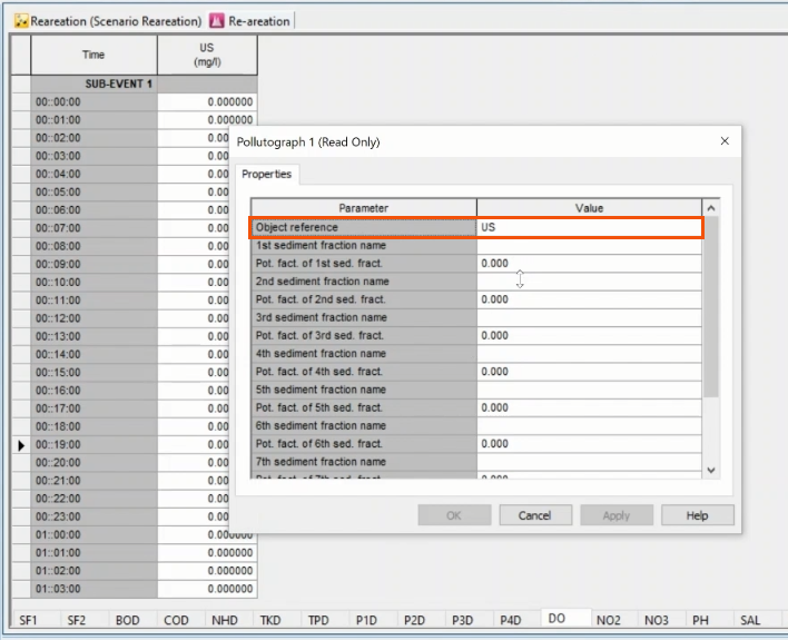
9. Right-click one of the values and select Profile properties.

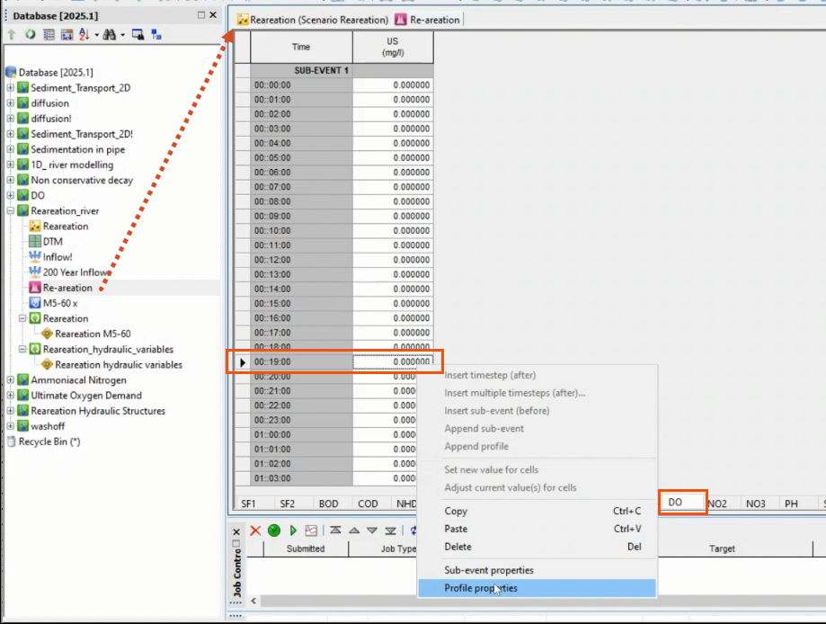
10. In the Pollutograph Properties dialog, assign the US node as the Object reference. This will apply the profile to the referenced upstream node in the water system.

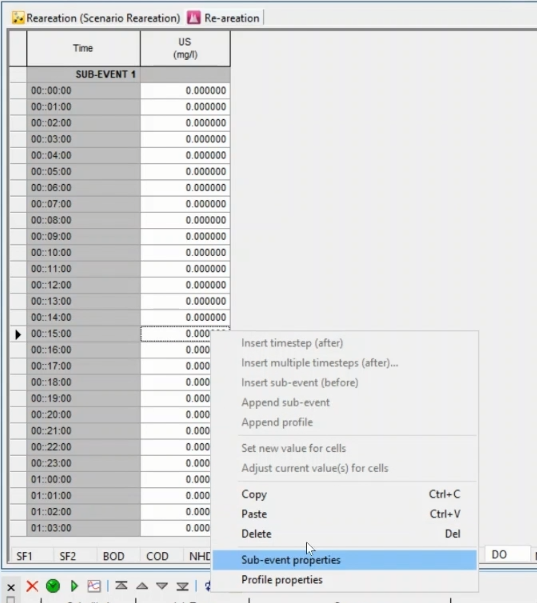
11. Right-click a value again and select Sub-event properties to further define the profile, as needed.
12. Validate and commit the scenario.

13. Back in the Database, right-click the Re-aeration run and select Open.
14. In the Run dialog, click Update to latest.

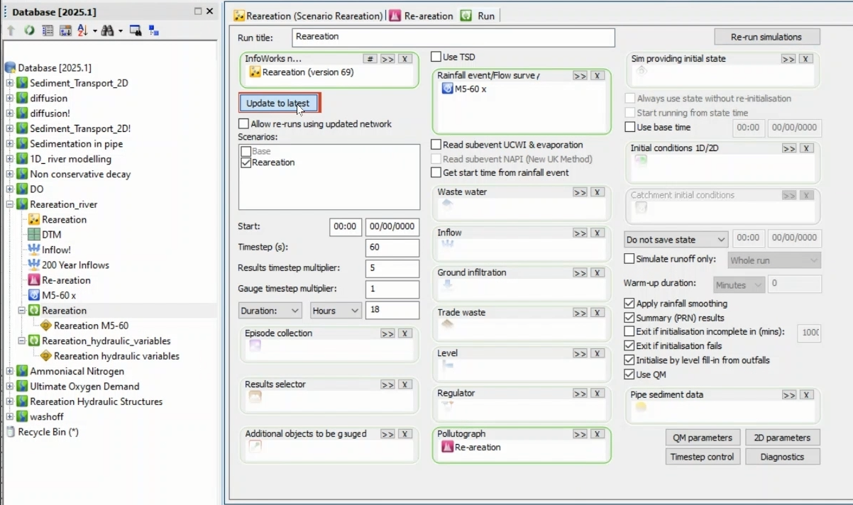
15. In the Scenarios list, verify that Reaeration is selected.
16. From the Database, drag the Re-aeration pollutograph into the Run dialog.

NOTE: To help ensure consistency, it is best practice to use the same run parameters specified in previous water quality saturated DO simulations.

17. Click QM Parameters.

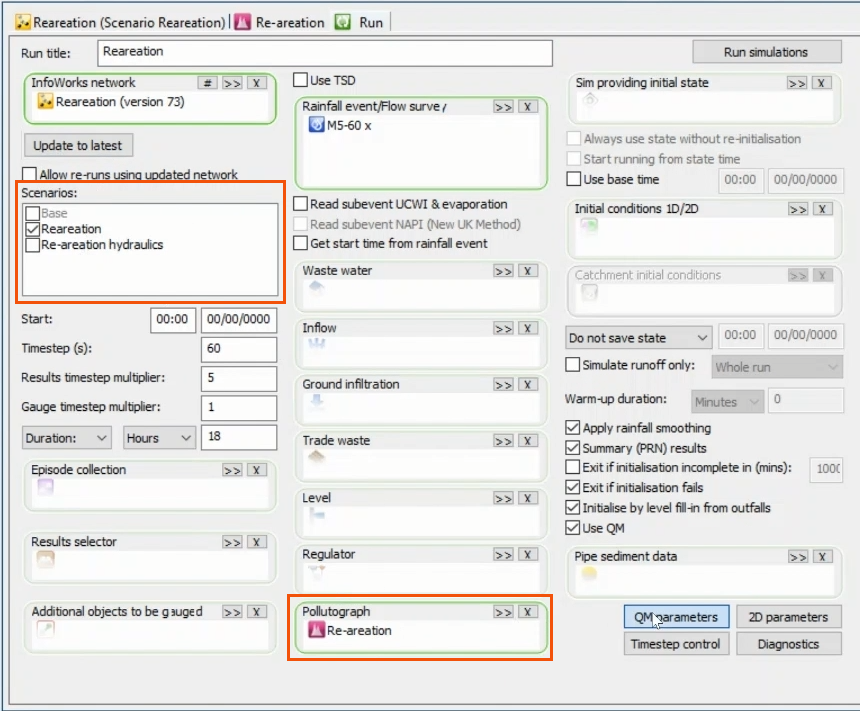
18. In the QM Parameters dialog, confirm the parameters and click OK.
19. Back in the Run dialog, click Run simulations.
20. In the Schedule Jobs dialog, verify the selections.
21. Click OK.

To create a second scenario to calculate reaeration based on hydraulics:

22. Create a new scenario and name it "Re-aeration hydraulics". OR In the toolbar, expand Reaeration and select Re-aeration hydraulics.
23. In the main menu, expand Model and select Model parameters > Water quality and sediment parameters.
24. Under Dissolved oxygen parameters, enable Calculate reaeration parameters.

NOTE: The Structure aeration coefficient is left at 0.000.

25. Validate and commit the scenario.
26. Back in the Database, open the Re-aeration_hydraulic_variables run.
27. In the Run dialog, click Update to latest.
28. In the Scenarios list, select Re-aeration hydraulics and deselect Reaeration.
29. Open QM parameters.

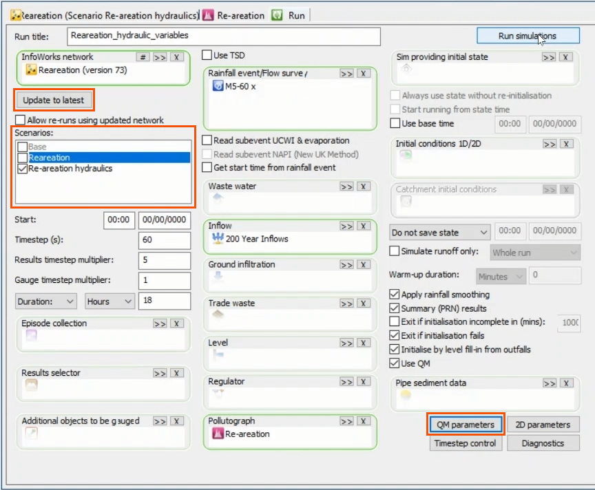
30. In the QM Parameters dialog, CONFIRM that the same determinants are selected.
31. Click OK.
32. In the Run dialog, click Run simulations.

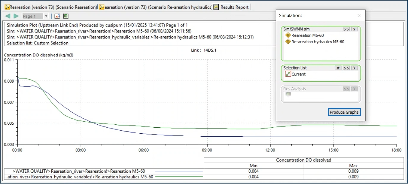
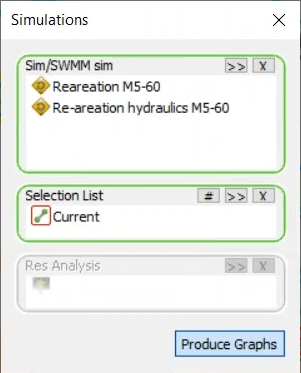
To plot both scenarios together:

33. In the GeoPlan, select the river reach.
34. Select Results > Graph reports > Simulation report.
35. From the Database, drag the two scenarios into the Simulations dialog.
36. For the Selection List, add the river reach, or Current selection.
37. Click Produce Graphs.

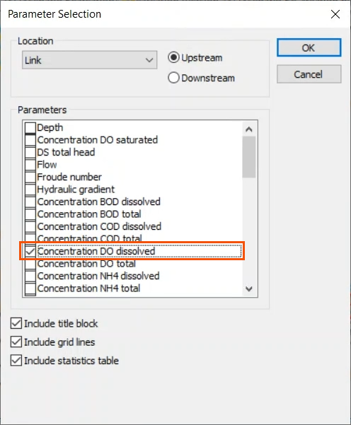
38. In the Parameter Selection dialog, select Concentration DO dissolved.
39. Click OK.

In this case, the reaeration rate was calculated both as a function of the predefined reaeration coefficient (0.03 meters per hour) and based on hydraulic variables, velocity and depth. The resulting plot shows a slight difference in the two calculations.