Simulate decaying pollutants
Step-by-step guide
Decaying determinants, or non-conservative determinants, are parameters with concentrations that change over time and distance due to both physical transport processes and chemical or biological reactions.
It is possible to model how non-conservative determinants behave in a water system:
- Degradation over time
- Reaction to substances
It is important to understand the various decay types and user-defined processes for modeling this behavior.
Non-conservative determinants exist in two primary forms:
- Dissolved pollutant
- Attached pollutant
Exceptions to this include parameters such as:
- Dissolved oxygen
- Salt
- pH levels
- Water temperature
Non-conservative pollutants can also react with other pollutants in the system.
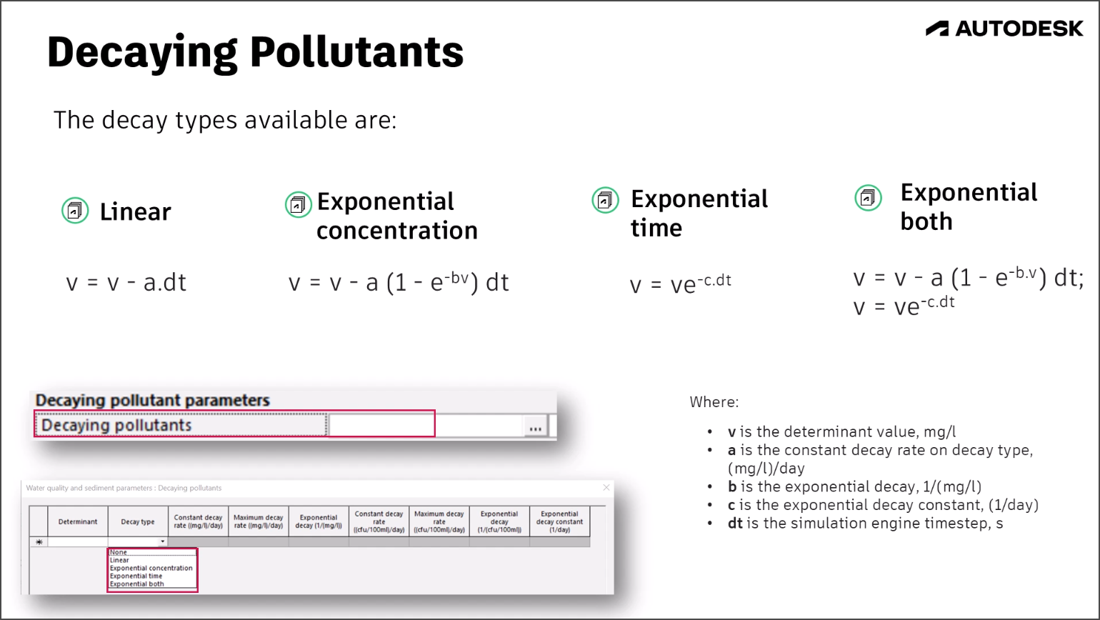
Methods to model the decay of pollutants in InfoWorks ICM:
- Linear decay: The pollutant decays at a constant rate.
- Exponential concentration: The decay rate depends on pollutant concentration.
- Exponential time: Uses a decay rate that is time-dependent.
- Exponential both: Combines concentration and time factors.
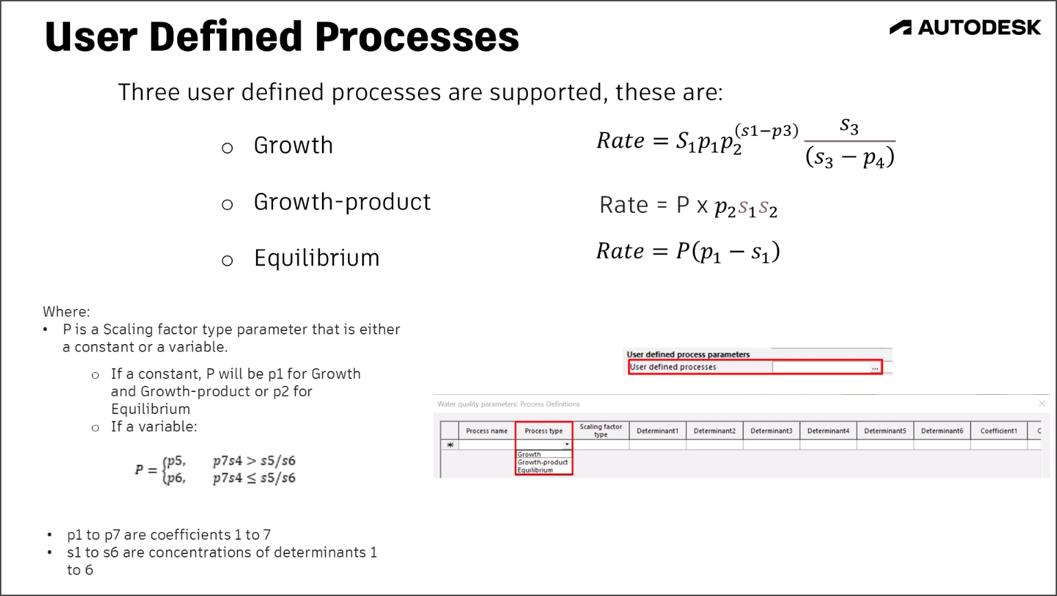
To simulate complex pollutant behaviors, custom processes can also be defined using specific equations and parameters. This allows for detailed customization to match real-world scenarios, including:
- Growth
- Growth-product
- Equilibrium
To introduce pollutant interactions by using decaying determinants:
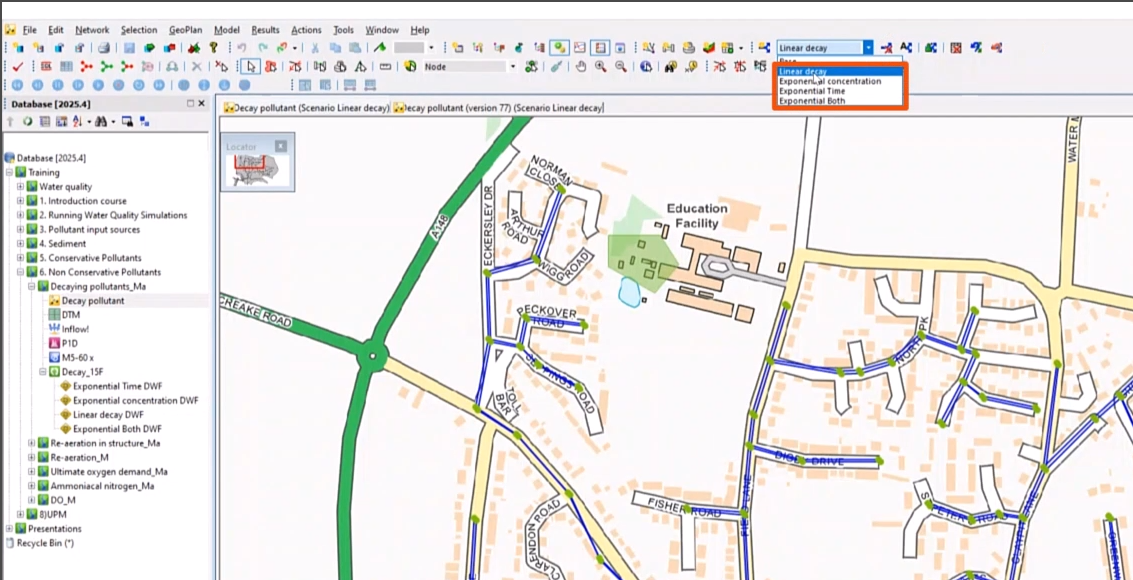
- Set up scenarios for the four decay options, as shown here in the Scenarios drop-down: Linear decay, Exponential concentration, Exponential time, and Exponential both.
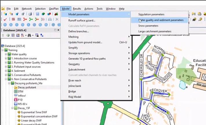
- Review the options to define these scenarios. Select Model > Model Parameters > Water quality and sediment parameters.
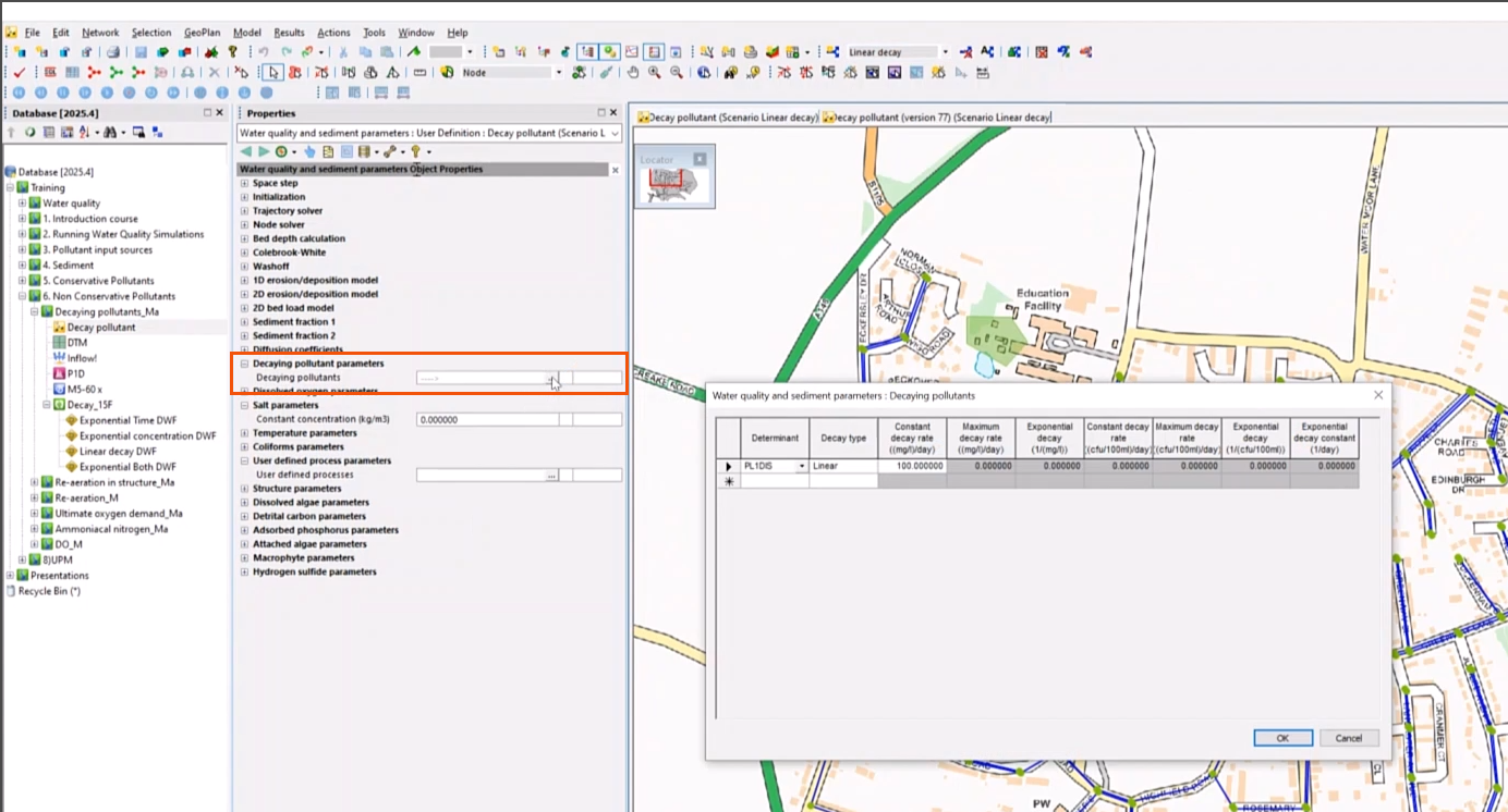
- In Properties, next to Decaying pollutants, click More (…).
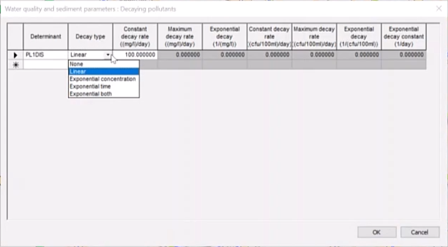
- In the Decaying pollutants dialog, in the list of Determinants, expand the Decay type drop-down to review the available types.
NOTE: For further customization, define the coefficient and equation to meet the needs of the specific scenario.
- In Properties, next to User defined processes, click More (…).
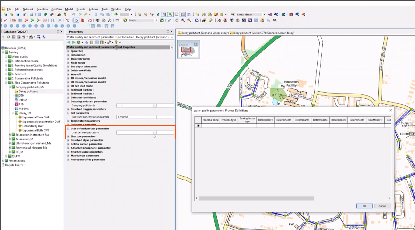
- In the Process Definitions dialog, expand the Process type to access the available options: Growth, Growth-product, and Equilibrium.
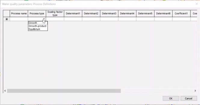
- Click OK.
Now, define the four scenarios:
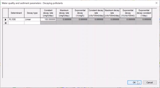
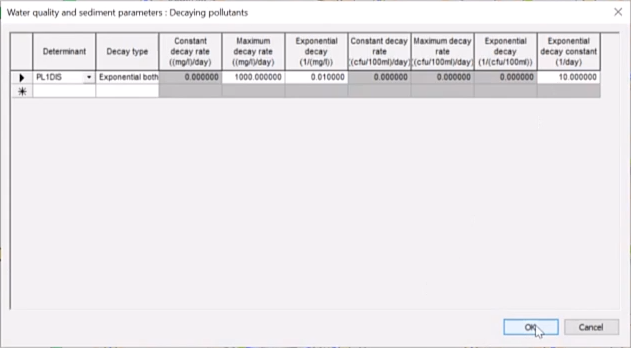
- For the Linear decay scenario, open the Decaying pollutants dialog.
- Specify the Determinant PL1.
- Set the Decay type to Linear.
- Enter a Constant decay rate of 100.
- Click OK.
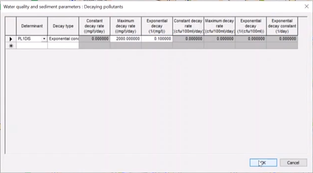
- For Exponential concentration, set the same Determinant and the corresponding Decay type.
- Set the Maximum decay rate to 2000.
- Set the Exponential decay rate to 0.1.
- Click OK.
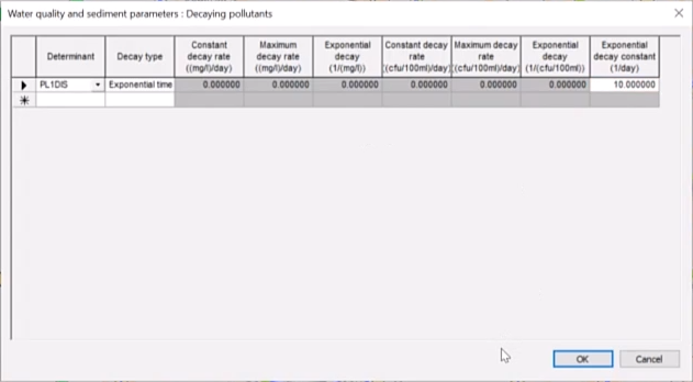
- For Exponential time, set the Exponential decay constant to 10.
- For Exponential both, set the Maximum decay rate to 1000.
- Set the Exponential decay to 0.01.
- Set the Exponential decay constant to 10.
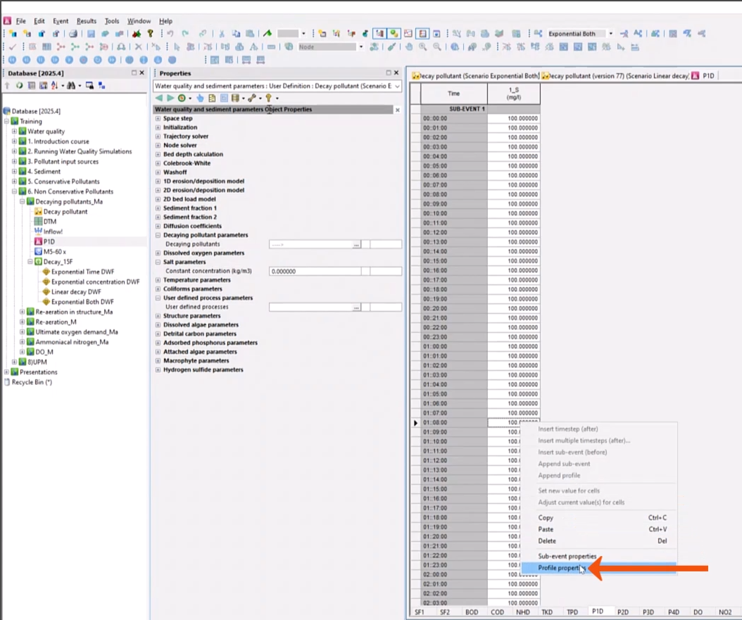
- Create a pollutograph by setting a value of 100 mg/l for determinant P1D, and then assign it to node 1_S. In this example, the pollutograph is already created:
- In the Explorer, right-click P1D and select Open.
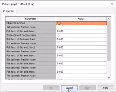
- To confirm that the 1_S node is assigned, on the P1D tab, right-click one of the profiles and select Profile Properties.
- In the Pollutograph properties dialog, confirm the Object reference.
- Click Cancel.
- Validate and commit the scenarios.
- From the Explorer, select the run to open the Run dialog, then expand it.
- If it is not already, drag and drop the P1D pollutograph into the Pollutograph field in the dialog.
- Select Use QM.
- Click QM Parameters.
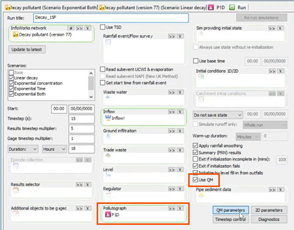
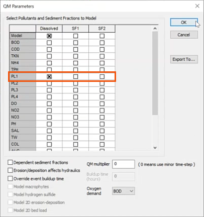
- In the QM Parameters dialog, ensure that PL1 is selected.
- Back in the Run dialog, click Run simulations to run all four scenarios.
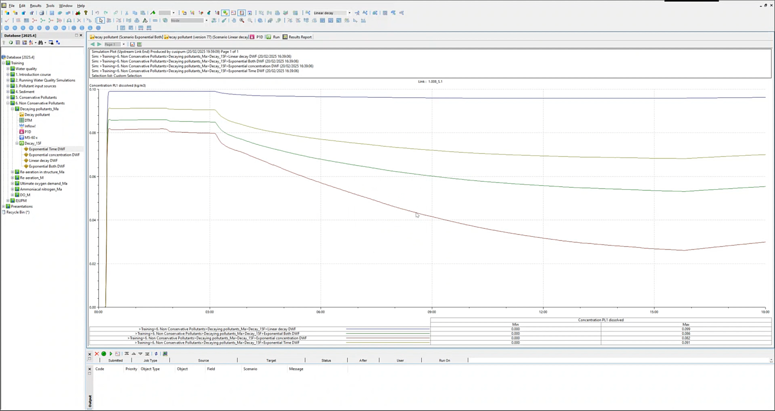
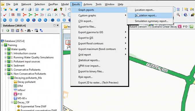
- Open the Linear decay scenario by selecting Results > Graph reports > Simulation report.
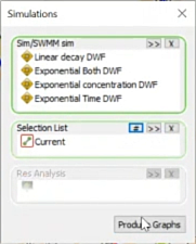
- From the Explorer, drag and drop the other three scenarios into the Simulations dialog to add them to the list.
- Under Selection List, select Current.
- Click Produce Graphs.
- In the Parameter Selection dialog, select Concentration PL1 dissolved.
- Click OK.
The graph displays the results of the four decay types changing over time.