Step-by-step guide
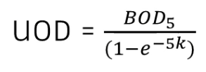
Ultimate Oxygen Demand (UOD) is the total oxygen required for microorganisms to decompose the organic matter present in water. There are two main types of UOD, but only one can be used at a time in the Dissolved Oxygen (DO) process.
- Biochemical Oxygen Demand (BOD) is the amount of dissolved oxygen needed by aquatic microorganisms to break down organic matter, including carbonaceous and nitrogenous oxygen demand. The most common form, BOD5, represents the oxygen consumed over a five-day period under standard conditions.
- Chemical Oxygen Demand (COD) is the total oxygen needed for the chemical oxidation of pollutants in water. This method measures organic matter in wastewater and natural waters using a strong chemical oxidizer in an acidic medium, providing a faster pollution assessment than BOD.
The key difference between BOD and COD is how oxygen demand is measured. BOD measures the oxygen used by microorganisms to break down organic matter, while COD measures the oxygen needed for chemical oxidation of pollutants.
Both values help assess water quality, but COD is typically faster, while BOD provides more insight into biological activity in a water sample.
BOD and COD can be specified as inputs from a variety of sources, and both are calculated as conservative pollutants.
Understanding ultimate oxygen demand is essential for monitoring and improving water quality. Oxygen demand can be measured as a function of either BOD or COD to track pollution levels, assess wastewater treatment efficiency, and protect aquatic ecosystems.
In ICM, the calculation of DO from BOD or COD follows similar steps. This example demonstrates the configuration for BOD.
To calculate DO from BOD:
- Create a pollutograph for BOD. Here, since one has already been created, right-click the BOD pollutograph and select Open.
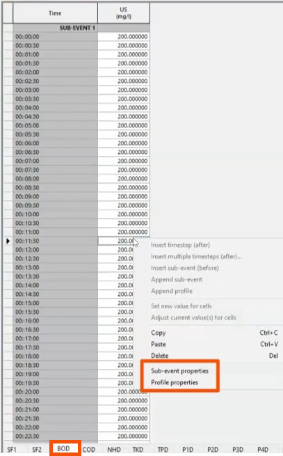
- On the BOD tab, define BOD as 200 milligrams per liter at the upstream node (US).
- In the BOD table, right-click any value and select Sub-event properties to review the selections for this configuration.
- Repeat this step to review the Profile properties.
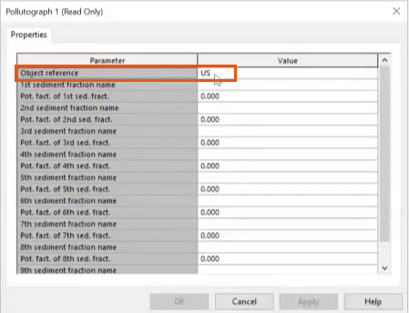
- In the Pollutograph Properties dialog, note that the US node is assigned as the Object reference.
Next, configure the run settings.
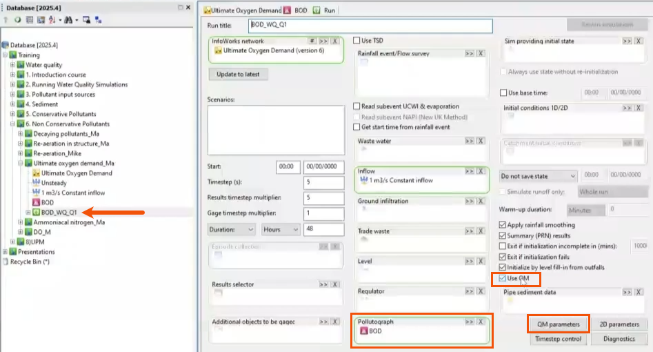
- In this case, from the Explorer window, open the Run dialog box for a simulation set up previously.
- Confirm that the BOD pollutograph has been dragged from the Database into the Pollutograph group box.
- Verify that Use QM is enabled.
- Click QM parameters.
- In the QM Parameters dialog, select the following pollutants: BOD, TKN, NH4, DO, NO2, and NO3.
IMPORTANT: When configuring BOD, it is essential to select these pollutants.
- In the Oxygen demand drop-down, select BOD. (When simulating chemical oxygen demand, select COD instead.)
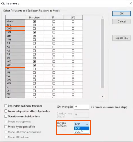
- Click OK.
- Back in the Run dialog, rename the simulation as needed.
- Click Run simulations.
Once the simulation is complete, plot the results to analyze the relationship between DO and BOD.
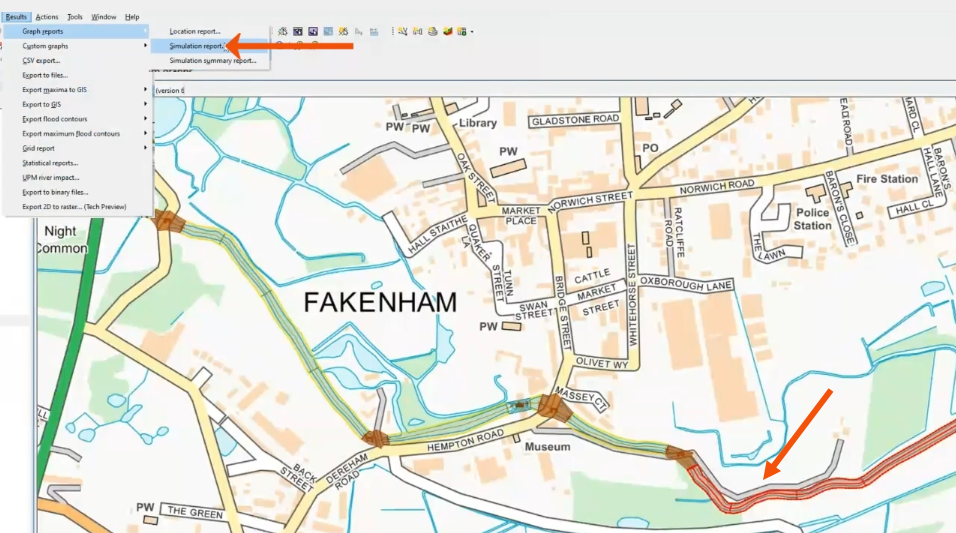
- In the GeoPlan, select the river reach.
- In the Results menu, select Graph reports > Simulation reports.
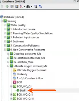
- From the Database, drag the completed simulation—in this case, DWF—into the Simulations dialog.
- Set the Selection List to Current.
- Click Produce Graphs.
- In the Parameter Selection dialog, select Concentration BOD dissolved and Concentration DO dissolved.
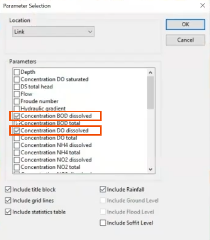
- Click OK.
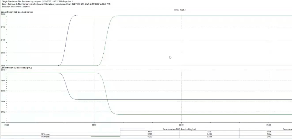
The resulting plots show that it takes about two to three hours for the pollutograph of BOD to flow from the node at which it is applied, node US, to the river reach.
When the BOD arrives in the river reach, there is an associated reduction in DO as the oxygen is used to decompose organic matter.


