Step-by-step guide
In InfoWorks ICM, sediment in pipes is treated differently by the hydraulic model and the water quality model.
Within a 1D pipe network, where the bed is fixed, erosion, and deposition in pipes occur in three stages, based on increasing flow velocity-induced shear stress (tau).
Erosion/deposition in pipes
There are different models for the two distinct layers of sediment in pipes: the passive layer and the active layer.
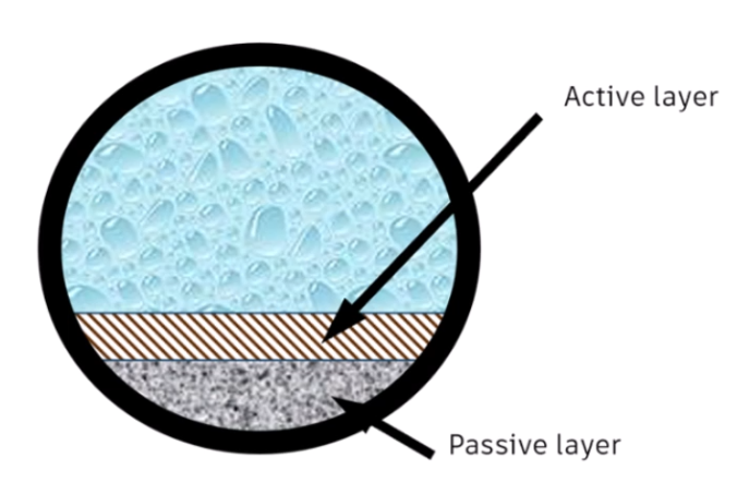
The passive layer is considered fixed and does not change during a simulation.
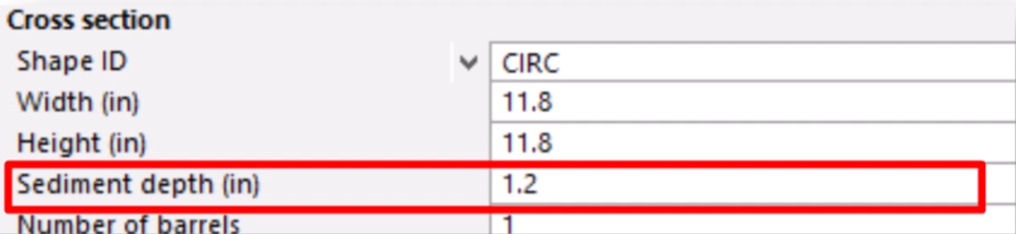
- Depth can be set in the Sediment depth field for each conduit.
- Behaves similarly to concrete—diminishes the hydraulic capacity of the pipe but has minimal effect on water quality.
The active layer consists of mobile sediment that can be eroded, transported, and deposited during a simulation.
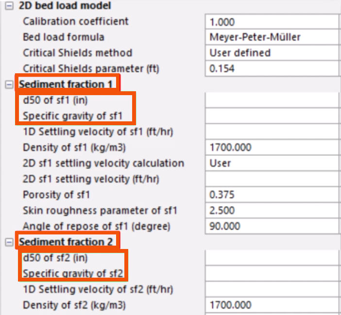
- Composed of one or two sediment fractions, each having different characteristics.
- Labeled Sediment Fraction 1 (SF1) and Sediment Fraction 2 (SF2) and defined by two parameters: D50, the average sediment particle size (with a default value of 0.04 mm) and Specific gravity (with a default value of 1.7).
Equations to calculate erosion/deposition
InfoWorks ICM supports three models for calculating erosion and deposition in pipes: Ackers-White, Velikanov, and KUL.
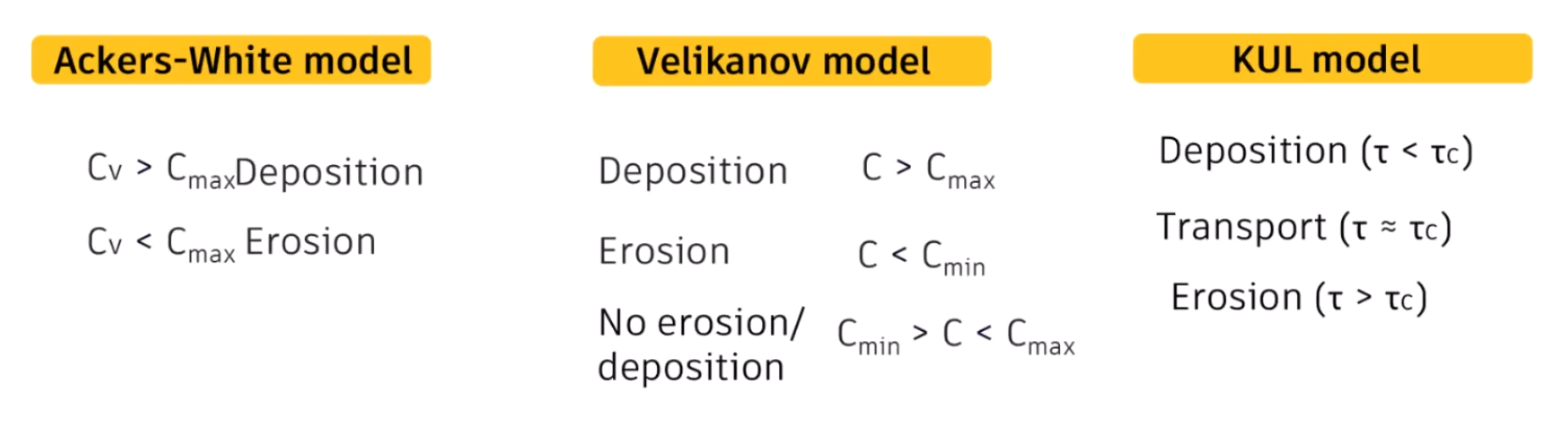
Ackers-White is the default model and uses a non-dimensional carrying capacity, Cν. According to this model:
- Sediment deposition occurs when the actual sediment concentration exceeds a maximum threshold, Cmax.
Deposition Cv > Cmax
Erosion occurs when the concentration is below Cmax, continuing until the concentration matches Cmax or the bed is fully eroded.
Erosion Cv < Cmax
The Velikanov model defines two critical concentrations: a minimum (Cmin) and a maximum (Cmax). According to this model:
- Erosion occurs if the flow concentration drops below Cmin, with the process aiming to restore Cmin.
Erosion C < Cmin
- Deposition takes place when the concentration surpasses Cmax, trying to stabilize at Cmax.
Deposition C > Cmax
- If the concentration remains between Cmin and Cmax, neither erosion nor deposition take place.
No erosion/deposition Cmin > C < Cmax
The KUL model uses a deposition-erosion criterion based on shear stress for sediment transport in sewers. According to this model:
- Deposition occurs when shear stress is below the critical level.
Deposition (τ < τc)
- Transport occurs at critical shear stress.
Transport (τ ≈ τc)
- Erosion occurs when shear stress exceeds the critical threshold.
Erosion (τ > τc)
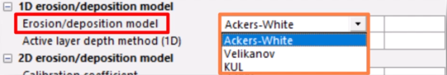
To select the model to use:
- Select Model > Model parameters > Water quality and sediment parameters.
- Navigate to the 1D erosion/deposition model group.
- For Erosion/deposition model, use the drop-down to select an option.
For all three models, the rate of deposition is defined by the settling velocity, which can also be specified in the model water quality parameters.
To incorporate the variable sediment depth from the water quality model into the hydraulic model:
- From the Run dialog box, select QM Parameters.
- In the QM Parameters dialog box, verify that Erosion/deposition affects hydraulics is selected. It is by default.
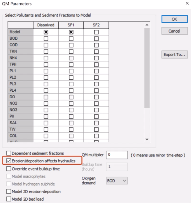
When selected:
- This is the only instance where water quality results will impact hydraulic results.
- The maximum deposition is 80% of the conduit height.
When deselected:
- Erosion and deposition do not alter the active layer thickness during the simulation.
- The maximum deposition is 10% of flow depth.
The only way to apply active sediment is to run a simulation. It is common practice to simulate a period of dry weather first and then save the final state file, which includes active sediment deposited in some of the pipes.
- To save the final state file, in the Run dialog box, select Save state at end.
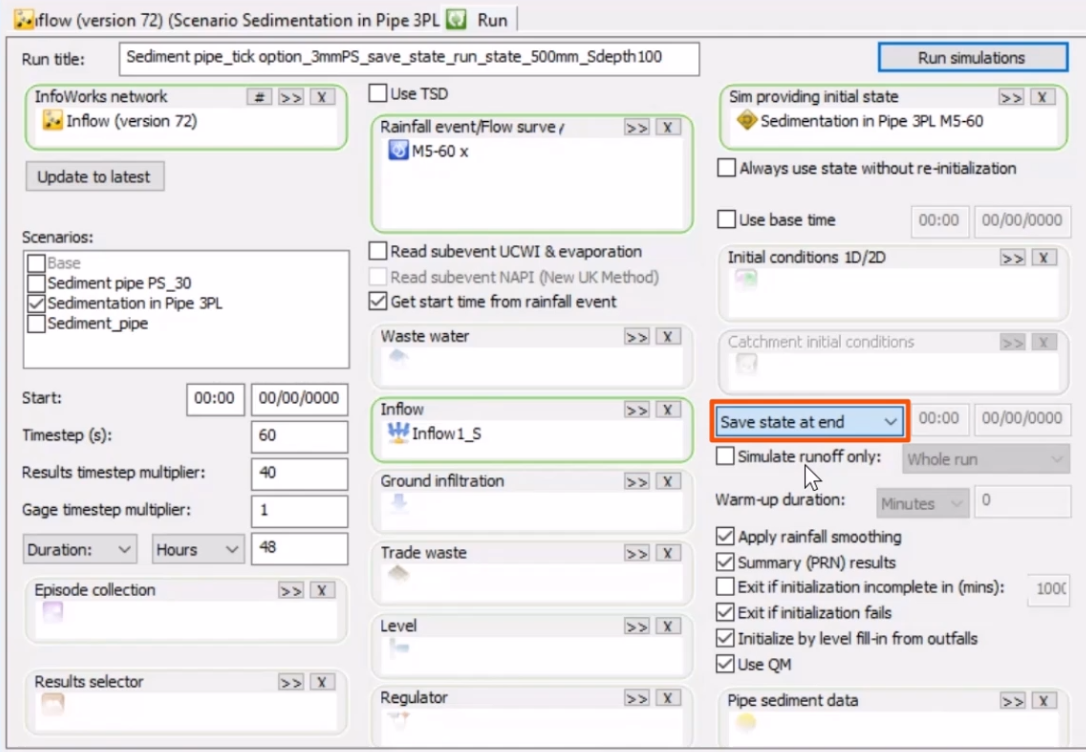
This state file can then be used as the starting point for storm analysis, during which this active sediment is re-eroded into the flow.
To average the two sediment fractions (SF1 and SF2) and model them together:
- Return to the QM Parameters dialog box.
- Select Dependent sediment fractions.
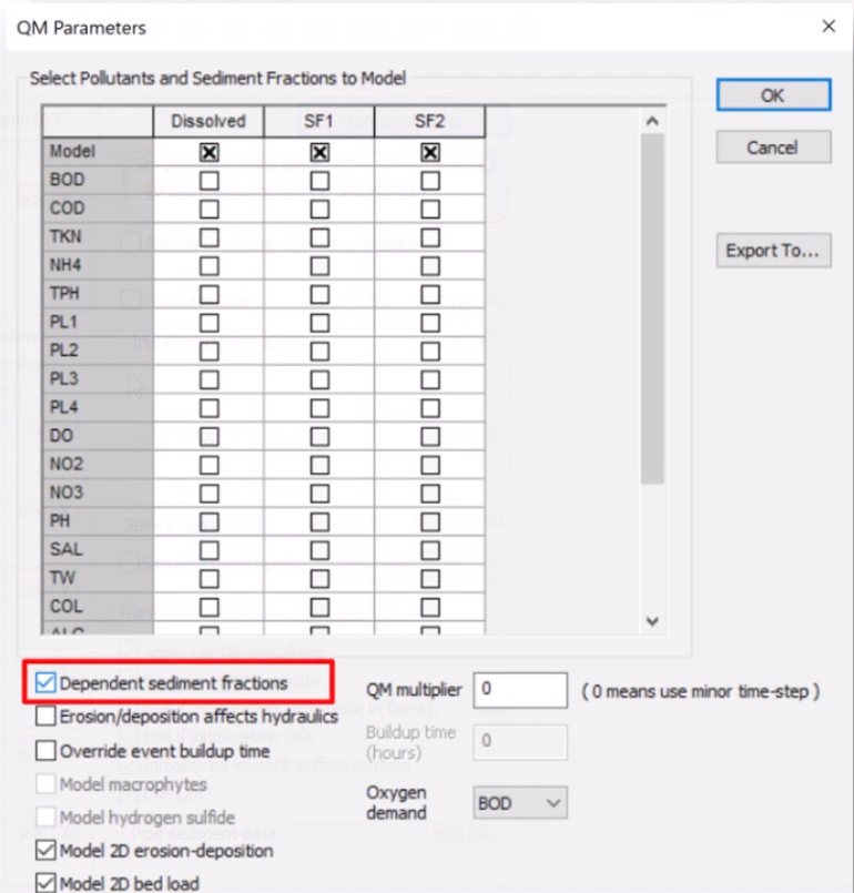
If this option is deselected, the two sediment fractions are modeled independently, with no interaction.
Results
Report the total sediment depth using graphs, tables, and long sections.
Note that results report the total sediment and not the various layers, whether active and passive, or SF1 and SF2, as shown below.
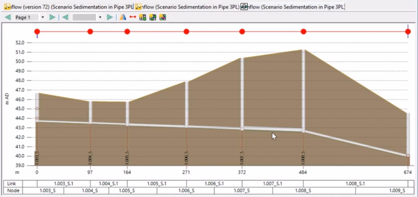
Initially, the sediment depth value is established, which remains constant and is not subject to erosion or deposition.
The example graph below shows the sediment concentration SF1 in a pipe, and the temporal change of concentration is depicted.
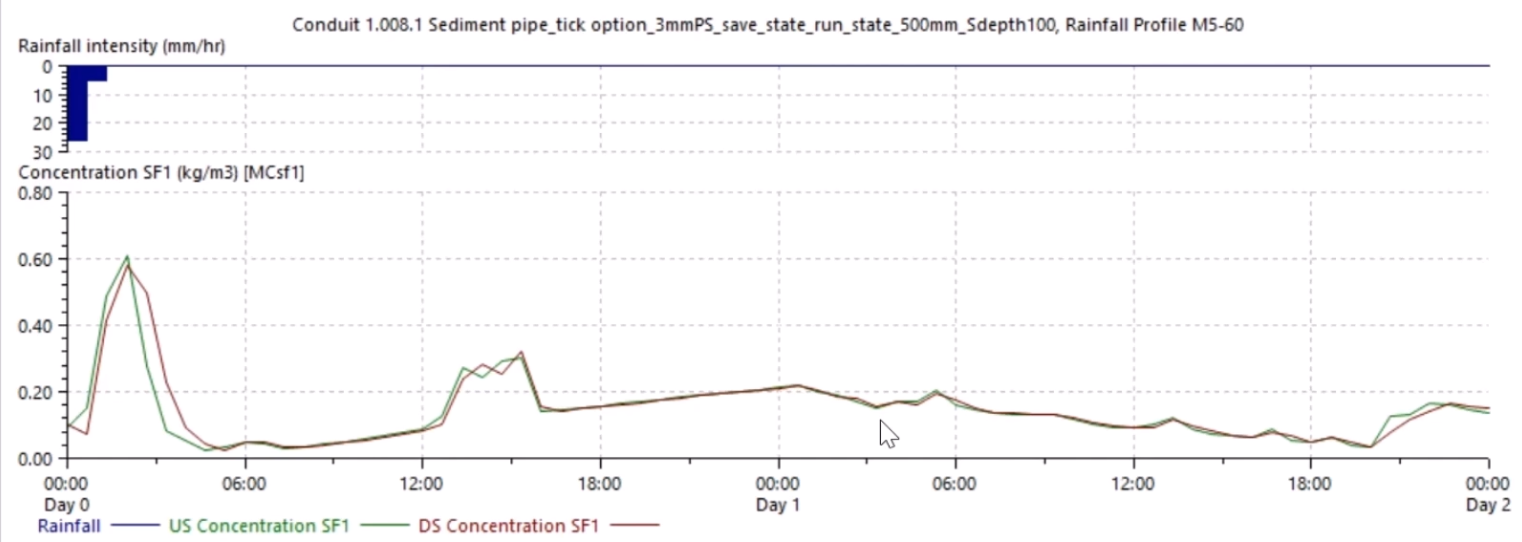
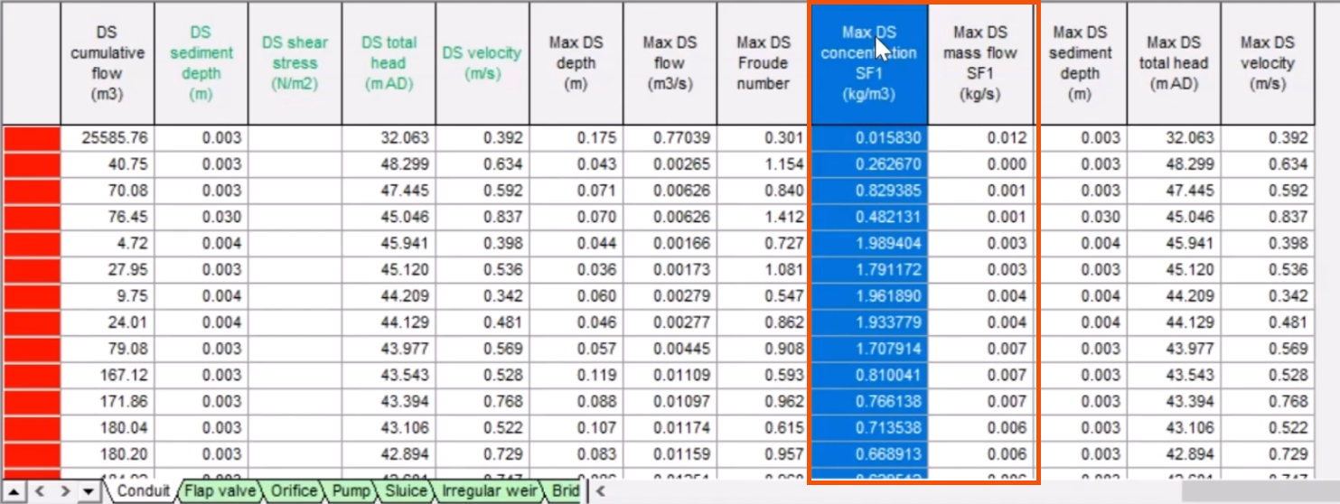
The maximum SF1 sediment concentration in kg/m3 and mass flow in kg/s values can be presented in a table for each pipe.