 Jon Holmes
The continuity equation says that water flowing into a pipe, channel, or junction must flow out, unless some of it is stored. Written as Q = A × V, it links flow rate, cross-sectional area, and velocity, and it’s one of the core principles behind hydraulic modeling. Here’s how it works and how modelers use it to balance flows in pipes, channels, and floodplains.
A heavy storm puts a drainage network to the test. Runoff pours into inlets and catch basins, water levels rise, and streets may begin to flood. For engineers trying to understand what happens next, one simple idea underpins the calculations: Water has to go somewhere.
The continuity equation expresses conservation of mass in fluid mechanics. It balances the mass entering and leaving a defined region with any change in stored mass. In hydraulics, it’s at work when a hydraulic model calculates pipe velocities, simulates a filling tank, or predicts where floodwater collects.
Most modelers won’t solve the equation by hand each time they run a simulation. The software handles that. But understanding what it’s balancing can help engineers make sense of the results and spot assumptions that call for a closer look.
Understand the continuity equation in fluid mechanics
Conservation of mass means mass cannot be created or destroyed. For a hydraulic system, that means incoming water must either leave the system or change the amount already stored there.
Engineers apply this principle to a defined region called a control volume. Picture a boundary around a tank, a stretch of river, or part of a floodplain. Any water crossing that boundary belongs in the balance.
For the hydraulic applications discussed here, water density can generally be treated as constant. The continuity equation then expresses a mass balance as a water-volume balance:
dS/dt = ∑Qin − ∑Qout
Here, S is stored volume, t is time, and Q is volumetric flow rate. The equation says that total inflow minus total outflow equals the rate of change in storage.
When more water comes in than goes out, storage increases. When more leaves than enters, storage decreases. If the two rates match, the stored volume stays the same.
That storage term matters. “Flow in equals flow out” works when storage isn’t changing. A filling tank follows the same conservation principle even though its inflow exceeds its outflow.
Relate flow rate and velocity with the continuity equation
The familiar Q = AV expression connects flow rate to the cross-sectional area available for water to move:
Q = A × V
Q is volumetric flow rate, also known as discharge. A is the cross-sectional area occupied by flowing water, and V is its average velocity through that area. Multiply square meters by meters per second, and the result is cubic meters per second.
Now picture a full pipe that narrows. Assume steady flow, constant water density, and no branches, leaks, or other additions or withdrawals between the two sections. The same volume must pass through each section every second:
A1V1 = A2V2
If the pipe carries 0.10 m³/s through an area of 0.05 m², its average velocity is 2 m/s. Halve that area to 0.025 m², and velocity doubles to 4 m/s. The water moves faster through the smaller opening to carry the same flow.
In US units: a pipe carrying 3 ft³/s through an area of 0.5 ft² has an average velocity of 6 ft/s. Halve the area to 0.25 ft², and velocity doubles to 12 ft/s.
That example assumes the flow rate stays the same. Installing a smaller pipe also changes resistance, which may change the flow the system can deliver. Continuity alone won’t tell you that response.
Engineers use this relationship when sizing pipes and checking velocities. Rearranging it as A = Q/V connects a design flow and candidate velocity to a required flow area. Pressure, friction losses, and other design requirements still need attention. In a partially full sewer or open channel, the area is the water-filled cross section, so it changes as water depth changes.
Keep junction flows in balance
At a water-distribution junction modeled without storage, all incoming water must leave through connected pipes or withdrawals such as customer demand.
Suppose two pipes bring in 12 L/s and 8 L/s. Customers draw 5 L/s at the junction, leaving 15 L/s to continue through a single outgoing pipe:
12 L/s + 8 L/s = 5 L/s + 15 L/s
In US units: 200 gpm + 100 gpm = 75 gpm + 225 gpm.
The customer demand belongs in the balance. Those 5 L/s have left the network, even though they haven’t passed into another modeled pipe.
With several outgoing pipes, the question gets more involved. Continuity sets the total that must leave, while hydraulic relationships involving pressure and resistance determine how it divides. Water-distribution software like InfoWater Pro and InfoWorks WS Pro solves junction flow conservation and pipe head-loss relationships together. InfoWater Pro’s hydraulic analysis is based on EPANET, the open-source modeling engine developed by the US EPA.
Close a pipe to test an outage, and that balance has to be recalculated using the remaining routes. Some flows may change direction, and pressures may fall. Conserving water doesn’t guarantee that each customer receives the requested supply. Pressure-dependent demand modeling helps represent how delivery changes when pressure is insufficient.
Watch the storage tank at work
A tank offers a clear view of what happens when inflow and outflow don’t match.
Imagine a tank receiving 30 L/s and releasing 20 L/s. The extra 10 L/s accumulates. If those rates stay constant for 10 minutes, the tank gains:
10 L/s × 600 seconds = 6,000 liters = 6 m³
In a tank with a constant plan area of 12 m², that raises the water level by 0.5 m.
In US units: a tank receiving 450 gpm and releasing 300 gpm gains 150 gpm. Over 10 minutes, that’s 1,500 gallons, or about 200 ft³. In a tank with a constant plan area of 100 ft², the level rises about 2 ft.
For a tank that changes shape with height, the model needs the corresponding relationship between stored volume and level.
That rising line on a tank-level graph reflects the accumulated difference between water entering and leaving. In an extended-period simulation, water distribution software updates tank levels using its calculated flows as it advances through time.
The same idea provides a useful check. If a tank keeps filling, more water must be entering than leaving over that period. If its level changes unexpectedly, review the connected flows, pump controls, and tank geometry before accepting the result.
Trace water from sewers to streets
During a storm, runoff can enter a sewer network faster than water leaves it. Storage increases, water levels rise, and pipes may become full and pressurized, or surcharged.
Surcharge doesn’t necessarily mean a flooded street. Water must rise high enough and have an available route to the surface, such as a manhole, before flooding occurs. How a model represents that route affects what happens to the excess water.
In a coupled 1D–2D model, water leaving the piped system becomes an input to the surface domain. Water may spread across a road, collect in a low spot, or flow back into the drainage system when system capacity becomes available. These exchanges are part of integrated catchment modeling, which connects drainage networks, rivers, and surface flows.
Continuity follows the water through the exchange. Looking at the sewer alone, water spilling onto the street is an outflow. Looking at the combined sewer and surface system, it’s an internal transfer.
For a modeler reviewing flood volumes, that distinction is useful. Does water leaving a manhole enter a modeled 2D area? Is it represented as ponded storage? Or does it leave the modeled system? The answer affects whether the simulation can show where that water travels and whether it returns.
Connect the continuity equation to hydraulic modeling
Flow rarely stays unchanged throughout a storm. Engineers call flow unsteady when conditions at a location vary over time.
A river reach, for example, can receive more water than it releases at a particular moment. The difference increases storage and changes water levels. A model has to track that balance along the reach and through time, using continuity alongside the equations managing water movement.
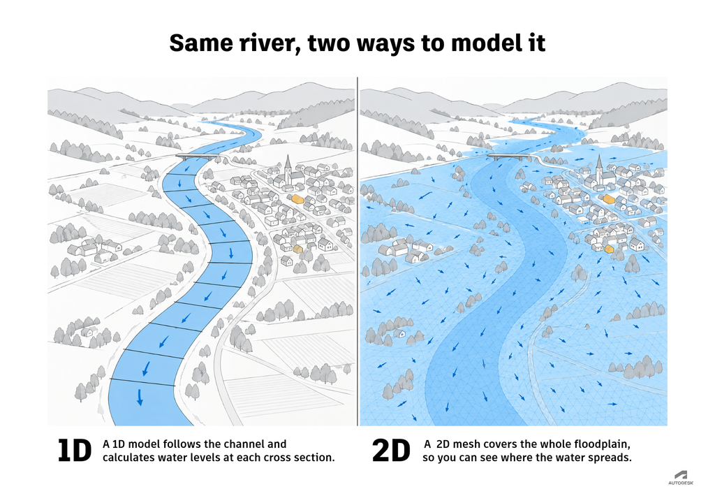
In InfoWorks ICM software’s 1D engine, the Saint-Venant equations pair conservation of mass with conservation of momentum. The mass equation accounts for water volume, while the momentum equation describes how forces change its motion. Together, these relationships help determine the changing flows and levels within the network.
InfoWorks ICM’s 2D engine uses the shallow-water equations, the 2D counterpart of the Saint-Venant equations, to represent depth-averaged flow in two horizontal directions. Both sets trace back to the Navier-Stokes equations, which describe fluid motion in general. The surface is divided into mesh elements, and the engine uses a formulation that conserves mass and momentum to calculate transfers between them. As an element gains or loses stored water, its depth changes. Connections from the 2D surface to the 1D network allow exchange between underground and surface flows.
The calculations differ between these settings, but the accounting remains familiar: Where, how much, and how fast did water enter, where did it leave, and how much is still there?
Check mass balance to build a better model
Understanding continuity gives engineers a practical way to interrogate unexpected results. A velocity that looks too high can prompt a check of flow and water-filled area. A tank that empties too quickly calls for a look at its net outflow or tank dimensions. A flood-volume result raises the question of where that water is represented.
Software diagnostics help check mass balance, too. Numerical calculations can create contradictions between incoming water, outgoing water, and storage changes. InfoWorks ICM includes node volume-balance checks that, when enabled, can trigger further iterations or smaller time steps if the specified tolerance is exceeded.
A good balance is one part of a credible model. Inaccurate geometry or inflows can still produce a water-conserving result. Once the accounting checks out, engineers can ask the next question: Does the model send that water to the right places?
Go deeper into hydraulic modeling
- Hydraulic modeling explained: a guide to 1D, 2D and integrated catchment modeling: See how continuity fits into the full modeling workflow, from data collection to calibration.
- 1D vs. 2D hydraulic modeling: how to choose for floods, dams, culverts and open channels: Learn how mass conservation applies in 1D and 2D models, and when to use each.
- HGL and EGL explained: See how a change in pipe diameter speeds up the flow and widens the gap between the hydraulic and energy grade lines.